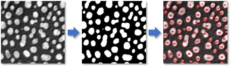
Notes on contours

QuPath aims to provide a new and powerful way to work with digital pathology images.

It’s intended to help a wide range of users: including pathologists, biologists, technicians and image analysts.

But QuPath doesn’t aim to replace existing open source image processing libraries.

For example, QuPath doesn’t contain its own code for applying a Gaussian filter. Or a median filter. Or for converting a binary image into contours - which is the topic of this post.

Rather, QuPath leaves these tasks to other implementations - which generally means either ImageJ or OpenCV.

The code within QuPath focusses instead on combining these basic building blocks to create custom algorithms to solve new problems, such as cell detection, tissue identification or superpixel generation - and package them up for application to whole slide images.

It is, of course, possible to write new implementations of basic image processing operations from scratch in QuPath. And sometimes that has been done; for example, to calculate texture features, or apply watershed transforms or morphological reconstruction.

But usually it’s avoided, if a suitable alternative can be found elsewhere.

Binary images to contours

At some point within an image analysis algorithm, it’s very common to end up with a binary (black and white) image representing one or more structures.

The next step is often then to trace around the boundaries of these structures, creating contours.

But it may not be obvious that there are different ways to approach this, and these can give different results.

Of particular importance here, OpenCV and ImageJ handle converting binary images into contours in quite different ways.

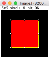
To investigate, we first consider the case where our binary image is extremely simple: showing just one foreground pixel in the middle.

Tracing contours with OpenCV

The common way to extract contours in OpenCV uses a method called findContours.

Here’s a short Python script that shows findContours in action:

import numpy as np
import cv2

# Create an image with 1 non-zero pixel in the center
bw = np.zeros((5, 5), np.uint8)
bw[2, 2] = 1
print(bw)

# Find & print the contours
_, contours, hierarchy = cv2.findContours(bw, cv2.RETR_CCOMP, cv2.CHAIN_APPROX_SIMPLE)
print('\nContours: ' + str(contours))

The following result is printed:

[[0 0 0 0 0]
 [0 0 0 0 0]
 [0 0 1 0 0]
 [0 0 0 0 0]
 [0 0 0 0 0]]

Contours: [array([[[2, 2]]], dtype=int32)]

From this, we can see that using OpenCV, the contour for a single pixel is a single point - represented by a single pair of coordinates.

Tracing contours with ImageJ

The following Groovy script applies the same contour-tracing idea as the Python script above, but this time using ImageJ.

It can be run through either QuPath & Fiji.

import ij.ImagePlus
import ij.plugin.filter.ThresholdToSelection
import ij.process.ByteProcessor

// Create an image with 1 non-zero pixel in the center
def ip = new ByteProcessor(5, 5)
ip.setf(2, 2, 255f)
ip.setThreshold(127.5, Double.MAX_VALUE, ByteProcessor.RED_LUT)

// Create ROI & print coordinates
def roi = new ThresholdToSelection().convert(ip)
def polygon = roi.getFloatPolygon()
println('X: ' + polygon.xpoints)
println('Y: ' + polygon.ypoints)

// Show the image, just to make sure
def imp = new ImagePlus("Small", ip)
imp.setRoi(roi)
imp.show()

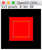
The result is shown below:

X: [3.0, 3.0, 2.0, 2.0]
Y: [3.0, 2.0, 2.0, 3.0]

From this, we can see that using ImageJ, the contour for a single pixel is a square - represented by four pairs of coordinates, one for each corner.

Getting bigger

Now to repeat the same thing, but with a 3x3 pixel region.

The Python code with OpenCV:

# Create an image with 3x3 non-zero pixels
bw = np.zeros((5, 5), np.uint8)
bw[1:4, 1:4] = 1
print(bw)

# Find & print the contours
_, contours, hierarchy = cv2.findContours(bw, cv2.RETR_CCOMP, cv2.CHAIN_APPROX_SIMPLE)
print(contours)

This does now result in a square:

[[0 0 0 0 0]
 [0 1 1 1 0]
 [0 1 1 1 0]
 [0 1 1 1 0]
 [0 0 0 0 0]]
[array([[[1, 1]],

       [[1, 3]],

       [[3, 3]],

       [[3, 1]]], dtype=int32)]

And the code for ImageJ:

import ij.ImagePlus
import ij.plugin.filter.ThresholdToSelection
import ij.process.ByteProcessor

// Create an image with 3x3 non-zero pixels
def ip = new ByteProcessor(5, 5)
ip.setRoi(1, 1, 3, 3)
ip.setValue(255)
ip.fill()
ip.resetRoi()
ip.setThreshold(127.5, Double.MAX_VALUE, ByteProcessor.RED_LUT)

// Create ROI & print coordinates
def roi = new ThresholdToSelection().convert(ip)
def polygon = roi.getFloatPolygon()
println('X: ' + polygon.xpoints)
println('Y: ' + polygon.ypoints)

// Show the image, just to make sure
def imp = new ImagePlus("Small", ip)
imp.setRoi(roi)
imp.show()

which also gives the corners of a square… but with different values:

X: [4.0, 4.0, 1.0, 1.0]
Y: [4.0, 1.0, 1.0, 4.0]

So which is right and which is wrong?

Clearly, both ‘make sense’ - they just represent different ways in which the image and its coordinates are interpreted.

One way to think of it is that, for OpenCV, (0, 0) represents the center of the top left pixel.

However, for ImageJ, (0, 0) represents the top left of the top left pixel.

However, even thought both are justifiable, the ImageJ interpretation fits much better with how QuPath works.

For example, consider the calculation of areas. QuPath does this based on vertices.

In the first case, the 1x1 pixel image, QuPath would use the coordinates from OpenCV and calculate an area of 0… i.e., nothing. But using the ImageJ representation, QuPath calculates the area of the square as being 1.

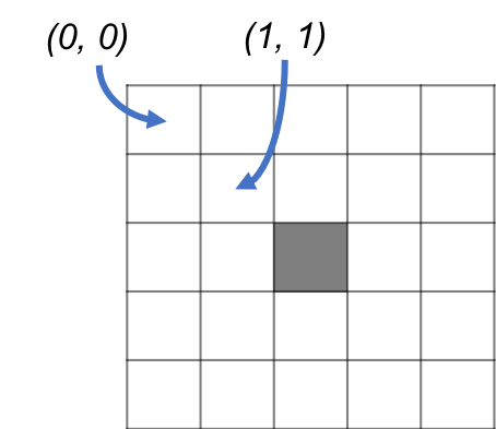
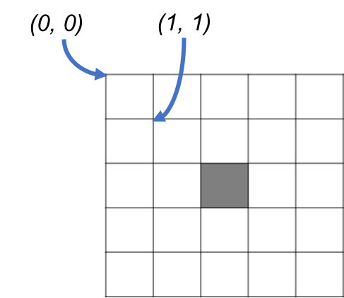
In the second case, the 3x3 pixel image, you can see for OpenCV that the maximum and minimum values for both x and y are 3 and 1. This implies a square where each side has length 2, and a total area of 4. But for ImageJ, the square has sides of length 3, and a total area of 9.

In other words, area calculations based on the ImageJ contours lead to the same results as would be obtained by ‘counting the pixels’ in the original binary image. But this is not true with the OpenCV contours.

This can be visualized as follows:

Using OpenCV contours - based on pixel centers

Using ImageJ contours - based on pixel edges

Why does this matter?

Most people should be able to use QuPath without needing to worry too much about the details.

But anyone who is developing new algorithms, or looking to export coordinates and use them in other software, ought to be aware of the differences in representation and what they can mean.

As it stands, the default Cell detection command in QuPath <= 0.1.2 uses ImageJ’s method of generating contours (and adds a bit of optional smoothing afterwards).

But there is also a lingering Watershed nucleus detection (OpenCV, experimental) command that uses OpenCV for cell detection. Currently, this command isn’t particularly good (and is likely to be removed in later versions of QuPath). Part of the reason it is less good may be the way in which it handles contours.

Personally, as I have started to use it more recently, I have grown to really like OpenCV and intend to use it more and more for processing and developing commands in the future… but may need to rely on a different method of generating contours rather than findContours, for the reasons described here.